Node functional API

The Node API features a simple implementation of computational graphs to develop complex reservoir computing architectures, similar to what can be found in other popular deep learning and differentiable calculus libraries. It is however simplified and made the most flexible possible by discarding the useless “fully differentiable operations” functionalities. If you wish to use learning rules making use of chain rule and full differentiability of all operators (stochastic gradient descent, for instance), ReservoirPy may not be the tool you need (actually, the whole paradigm of reservoir computing might arguably not be the tool you need).

What is a Node?

In ReservoirPy, all operations are Nodes. For instance, imagine you want to build an Echo State Network (ESN). An ESN is made of a reservoir, a pool of randomly connected neurons with recurrent connexions, and a readout, a layer of linear neurons connected with the neurons of the reservoir. The readout connections are moreover equipped with a learning rule such as ridge regression.

To define an ESN in ReservoirPy, we therefore need to connect two nodes in a graph: a Reservoir node and a Ridge node. The graph defines that the reservoir internal states must be given as input to the readout.

These two nodes give access to all characteristics of the reservoir and the readout we define for the task: their parameters, their hyperparameters, their states, their functions, and so on.

In the following guide, you will learn more about how to work with Node objects. If you want to learn more about how to define computational graphs of nodes, you can read From Nodes to Models.

What is a Node, really?

In a computational graph, each operation is represented by a Node. A node is able to apply the operation it holds on any data reaching it through all the connections with other nodes in the graph. Within ReservoirPy, we define a Node as a simple object holding a function and an internal state (Fig. 1):

Fig. 1 The most simple schema of a Node.

Here, a node is given a function \(f\), called a forward function, and an internal state \(s[t]\). Notice how this state depends on a mysterious variable \(t\). Well, this is just a discrete representation of time. Indeed, all operations in ReservoirPy are recurrent: the forward function \(f\) is always applied on some data and on its own previous results, stored in the state \(s\) (Fig. 2).

To summarize, a node performs operations that can be mathematically expressed as (1):

(1)\[s[t+1] = f(s[t], x[t])\]

where \(x[t]\) represents some input data arriving to the node at time \(t\).

Fig. 2 A Node is used to executes the forward function \(f\), which computes its next state \(s[t+1]\) given the current state of the Node \(s[t]\) and some input data \(x[t]\).

Accessing state

In ReservoirPy, a node internal state is accessible through the state() method:

s_t0 = node.state()

The state is always a ndarray vector, of shape (1, ndim), where ndim is the dimension of the node internal state.

To learn how to modify or initialize a node state, see Reset or modify reservoir state.

Applying node function and updating state

And to apply the forward function \(f\) to some input data, one can simply use the call() method of a node, or directory call the node on some data:

# using 'call'
s_t1 = node.call(x_t0)
# using node as a function
s_t1 = node(x_t0)

This operation automatically triggers the update of the node internal state (Fig. 3):

# node internal state have been updated from s_t0 to s_t1
assert node.state() == s_t1

To learn how to modify this automatic update, see Reset or modify reservoir state.

Fig. 3 Calling a Node returns next state value \(s[t+1]\) and updates the node internal state with this new value.

Parametrized nodes

It is also possible to hold parameters in a node, to change the behaviour of \(f\). In this case, \(f\) becomes a parametrized function \(f_{p, h}\). The parameters \(p\) and \(h\) are used by the function to modify its effect. They can be, for instance, the synaptic weights of a neural network, or a learning rate coefficient. If these parameters evolve in time, through learning for instance, they should be stored in \(p\). We call them parameters. If these parameters can not change, like a fixed learning rate, they should be stored in \(h\). We call them hyperparameters.

Fig. 4 A Node can also hold parameters and hyperparameter to parametrize \(f\).

A node can therefore be more generally described as (2):

(2)\[s[t+1] = f_{p,h}(s[t], x[t]) = f(s[t], x[t], p, h)\]

Parameters and hyperparameters of the node can be accessed through the Node.params and Node.hypers attributes:

In [1]: node.params
Out [1]: {"param1": [[0]], "param2": [[1, 2, 3]]}

In [2]: node.hypers
Out [2]: {"hyper1": 1.0, "hyper2": "foo"}

They can also directly be accessed as attributes:

In [3]: node.param2
Out [3]: [[1, 2, 3]]

In [4]: node.hyper1
Out [4]: 1.0

Naming nodes

Nodes can be named at instantiation.

node = Node(..., name="my-node")

Naming your nodes is a good practice, especially when working with complex models involving a lot of different nodes.

Warning

All nodes created should have a unique name. If two nodes have the same name within your environment, an exception will be raised.

Be default, nodes are named Class-#, where Class is the type of the node and # is the unique number associated with this instance of Class.

Running nodes on timeseries or sequences

Reservoir Computing is usually applied to problems where timing of data carries relevant information. This kind of data is called a timeseries. As all nodes in ReservoirPy are recurrently defined, it is possible to update a node state using a timeseries as input instead of one time step at a time. The node function will then be called on each time steps of the timeseries, and the node state will be updated accordingly (Fig. 5):

Fig. 5 A Node can apply its function on some timeseries while updating its state at every time step.

To apply a Node on a timeseries, you can use the run() method:

# X = [x[t], x[t+1], ... x[t+n]]
states = node.run(X)
# states = [s[t+1], s[t+2], ..., s[t+n+1]]

An example using Reservoir node

Let’s use the Reservoir class as an example of node. Reservoir class is one of the cornerstone of reservoir computing tools in ReservoirPy. It models a pool of leaky integrator rate neurons, sparsely connected together. All connections within the pool are random, and neurons can be connected to themselves. The forward function of a Reservoir node can be seen in equation (3).

(3)\[ s[n+1] = (1 - lr) \cdot s[t] + \alpha \cdot f(W_{in} \cdot x[n] + W \cdot s[t])\]

Internal state of the reservoir \(s[t]\) is in that case a vector containing the activations of all neurons at timestep \(t\). The forward function is parametrized by an hyperparameter \(lr\) (called leaking rate) and two matrices of parameters \(W\) and \(W_{in}\), storing the synaptic weights of all neuronal connections. Connections stored in \(W\) are represented using in figure Fig. 6, and connections stored in \(W_{in}\) are represented using .

Fig. 6 A Reservoir. Internal state of the node is a vector containing activations of all neurons in the reservoir.

To instantiate a Reservoir, only the number of units within it is required. Leaking rate will have in that case a default value of 1, and \(W\) and \(W_{in}\) will be randomly initialized with a 80% sparsity.

In [5]: from reservoirpy.nodes import Reservoir

In [6]: nb_units = 100  # 100 neurons in the reservoir

In [7]: reservoir = Reservoir(nb_units)

Parameters and hyperparameters are accessible as attributes:

In [8]: print(reservoir.lr)  # leaking rate
1.0

Now, let’s call the reservoir on some data point \(x[t]\), to update its internal state, initialized to a null vector. We first create some dummy timeseries X:

In [9]: X = np.sin(np.arange(0, 10))[:, np.newaxis]

Notice that all nodes require data to be 2-dimensional arrays, with first axis representing time and second axis representing features. We can now call the reservoir on some data, to update its internal state as shown below. Reservoir state is accessible using its state() method.

In [10]: s_t1 = reservoir(X[0])

In [11]: assert np.all(s_t1 == reservoir.state())

Fig. 7 A Reservoir is called on some data point \(x[t]\), which activates the pool of neurons to update their state according to equation (3).

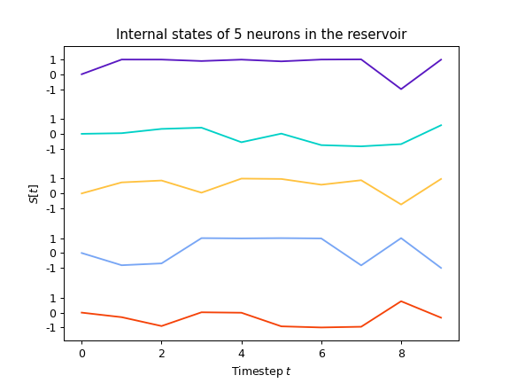
We can also retrieve all activations of the reservoir on the full timeseries, using run():

In [12]: S = reservoir.run(X)

The plot below shows these activations for 5 neurons in the reservoir, over the entire timeseries:

Learn more

Now that you are more familiar with the basic concepts of the Node API, you can see:

• From Nodes to Models on how to connect nodes together to create Model objects,

• Learning rules on how to make your nodes and models learn from data,

• Feedback connections on how to create feedback connections between your nodes,

• Create your own Node on how to create your own nodes, equipped with custom functions and learning rules.

References

ReservoirPy Node API was heavily inspired by Explosion.ai Thinc functional deep learning library [1], and Nengo core API [2]. It also follows some scikit-learn schemes and guidelines [3].

[1]

Thinc website

[2]

Nengo website

[3]

scikit-learn website