Learning rules#
Reservoir Computing techniques allow the use of a great variety of learning mechanisms to solve specific tasks. In ReservoirPy, these learning rules are sorted in two categories: offline learning rules and online learning rules.
Nodes can be equipped with such learning rules, and learning can be triggered by using their,
fit() (offline learning) and partial_fit() (online learning) methods.
Offline learning rules - Linear regression#
Offline learning rules are the most common learning rules in machine learning. They include gradient descent and linear regression amongst others. Within the Reservoir Computing field, linear regression is probably the simplest and the more used way of training an artificial neural network.
Linear regression is said to be an offline learning rule because parameters of the linear regression model are learned given all available samples of data and all available samples of target values. Once the model is learned, it can not be updated without training the model on the whole dataset another time. Training and data gathering happen in two separate phases.
Linear regression is implemented in ReservoirPy through the Ridge node. Ridge node is equipped with a
regularized linear regression learning rule, of the form (5):
Where \(X\) is a series of inputs, and \(Y\) is a series of target values that the network must learn to
predict. \(\lambda\) is a regularization
parameter used to avoid overfitting. In most cases, as the Ridge node will be used within an Echo State
Network (ESN), \(X\) will represent the series of activations of a Reservoir node over a timeseries.
The algorithm will therefore compute a matrix of neuronal weights \(W_{out}\) (and a bias term)
such as predictions can be computed using equation (6).
\(W_{out}\) (and bias) is stored in the node Node.params attribute.
which is the forward function of the Ridge node. \(y[t]\) represents the state of the Ridge neurons at step \(t\), and also the predicted value given the input \(x[t]\).
Offline learning with fit()#
Offline learning can be performed using the fit() method.
In the following example, we will use the Ridge node.
We start by creating some input data X and some target data Y that the model has to predict.
In [1]: X = np.arange(100)[:, np.newaxis]

In [2]: Y = np.arange(100)[:, np.newaxis]
Then, we create a Ridge node. Notice that it is not necessary to indicate the number of neurons in that
node. ReservoirPy will infer it from the shape of the target data.
In [3]: from reservoirpy.nodes import Ridge

In [4]: ridge = Ridge().fit(X, Y)
We can access the learned parameters looking at the Wout and bias parameter of the node.
In [5]: print(ridge.Wout, ridge.bias)
[[1.]] [0.]
As X and Y where the same timeseries, we can see learning was successful: the node has learned the identity
function, with a weight of 1 and a bias of 0.
Ridge regression can obviously handle much more complex tasks, such as chaotic attractor modeling or timeseries forecasting, when coupled with a reservoir inside an ESN.
Offline learning with fit()#
Models also have a fit() method, working similarly to the one of the Node class presented above.
The fit() method can only be used if all nodes in the model are offline nodes, or are not trainable.
If all nodes are offlines, then the fit() method of all offline nodes in the model will be called
as soon as all input data is available. If input data for an offline node B comes from another offline node A,
then the model will fit A on all available data, then run it, and finally resume training B.
As an example, we will train the readout layer of an ESN using linear regression. We first create some toy dataset: the task we need the ESN to perform is to predict the cosine form of a wave given its sine form.
In [6]: X = np.sin(np.linspace(0, 20, 100))[:, np.newaxis]

In [7]: Y = np.cos(np.linspace(0, 20, 100))[:, np.newaxis]
Then, we create an ESN model by linking a Reservoir node with a Ridge node. The
Ridge node will be used as readout and trained to learn a mapping between reservoir states
and targeted outputs. We will regularize its activity using a ridge parameter of \(10^{-3}\). We will also tune
some of the reservoir hyperparameters to obtain better results.
We can then train the model using fit().
In [8]: from reservoirpy.nodes import Reservoir, Ridge

In [9]: reservoir, readout = Reservoir(100, lr=0.2, sr=1.0), Ridge(ridge=1e-3)

In [10]: esn = reservoir >> readout

In [11]: esn.fit(X, Y)
Out[11]: Model(Reservoir(units=100, lr=0.2, input_dim=1), Ridge(ridge=0.001, input_dim=100, output_dim=1))
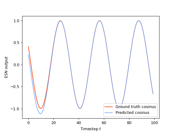
During that step, the reservoir has been run on the whole timeseries, and the resulting internal states has been used to perform a linear regression between these states and the target values, learning the connection weights between the reservoir and the readout. We can then run the model to evaluate its predictions:
In [12]: X_test = np.sin(np.linspace(20, 40, 100))[:, np.newaxis]

In [13]: predictions = esn.run(X_test)
Online learning rules#
As opposed to offline learning, online learning allows to learn a task using only local information in time. Example of online learning rules are Hebbian learning rules, Least Mean Squares (LMS) algorithm or Recurrent Least Squares (RLS) algorithm.
These rules can update the parameters of a model one sample of data at a time, or one episode at a time to borrow vocabulary used in the Reinforcement Learning field. While most deep learning algorithms can not used such rules to update their parameters, as gradient descent algorithms requires several samples of data at a time to obtain convergence, Reservoir Computing algorithms can use this kind of rules. Indeed, only readout connections need to be trained. A single layer of neurons can be trained using only local information (no need for gradients coming from upper layers in the models and averaged over several runs).
Online learning with partial_fit()#
Online learning can be performed using the partial_fit() method.
In the following example, we will use the RLS node, a single layer of neurons equipped with
an online learning rule called the Recursive Least Square (RLS) algorithm.
We start by creating some input data X and some target data Y that the model has to predict.
In [14]: X = np.arange(100)[:, np.newaxis]

In [15]: Y = np.arange(100)[:, np.newaxis]
Then, we create an RLS node. Notice that it is not necessary to indicate the number of neurons in that
node. ReservoirPy will infer it from the shape of the target data.
In [16]: from reservoirpy.nodes import RLS

In [17]: rls = RLS()
The partial_fit() method can be used as the call method of a Node. Every time the method is called, it updates
the parameter of the node along with its internal state, and return the state.
In [18]: s_t1 = rls.partial_fit(X[:10], Y[:10])

In [19]: print("Parameters after first update:", rls.Wout, rls.bias)
Parameters after first update: [[0.9272]] [0.5447]

In [20]: s_t1 = rls.partial_fit(X[10:], Y[10:])

In [21]: print("Parameters after second update:", rls.Wout, rls.bias)
Parameters after second update: [[0.9855]] [1.1068]
The partial_fit() method can also be called on a timeseries of variables and targets, in a similar way to
what can be done with the run() function. All states computed during the training will be returned
by the node.
In [22]: rls = RLS()

In [23]: S = rls.partial_fit(X, Y)
As the parameters are updated incrementally, we can see convergence of the model throughout training, as opposed to offline learning where parameters can only be updated once, and evaluated at the end of the training phase. We can see that convergence is really fast. Only the first timesteps of output display visible errors:
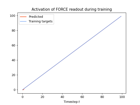
We can access the learned parameters looking at the Wout and bias parameter of the node.
In [24]: print(rls.Wout, rls.bias)
[[0.9855]] [1.1068]
As X and Y where the same timeseries, we can see learning was successful: the node has learned the identity
function, with a weight of 1 and a bias close to 0.
Online learning with partial_fit()#
Models also have a partial_fit() method, working similarly to the one of the Node class presented above.
The partial_fit() method can only be used if all nodes in the model are online nodes, or are not trainable.
If all nodes are online, then the partial_fit() methods of all online nodes in the model will be called in the
topological order of the graph defined by the model. At each timesteps, online nodes are trained, called, and their
updated states are given to the next nodes in the graph.
As an example, we will partially fit the readout layer of an ESN using RLS learning. We first create some toy dataset: the task we need the ESN to perform is to predict the cosine form of a wave given its sine form.
In [25]: X = np.sin(np.linspace(0, 20, 100))[:, np.newaxis]

In [26]: Y = np.cos(np.linspace(0, 20, 100))[:, np.newaxis]
Then, we create an ESN model by linking a Reservoir node with an RLS node. The
RLS node will be used as readout and trained to learn a mapping between reservoir states
and targeted outputs. We will tune some of the reservoir hyperparameters to obtain better results.
We can then train the model using partial_fit().
In [27]: from reservoirpy.nodes import Reservoir, RLS

In [28]: reservoir, readout = Reservoir(100, lr=0.2, sr=1.0), RLS()

In [29]: esn = reservoir >> readout

In [30]: predictions = esn.partial_fit(X, Y)
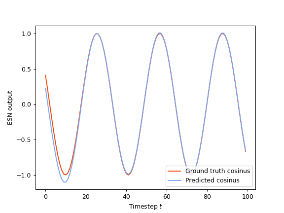
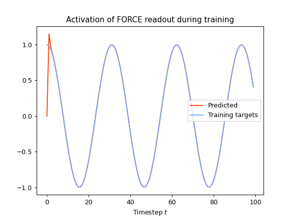
During that step, the reservoir has been trained on the whole timeseries using online learning. We can have a look at the outputs produced by the model during training to evaluate convergence:
We can then run the model to evaluate its predictions:
In [31]: X_test = np.sin(np.linspace(20, 40, 100))[:, np.newaxis]

In [32]: predictions = esn.run(X_test)