Advanced features#
This tutorial covers usage of advanced features of ReservoirPy for Reservoir Computing architectures:
Input-to-readout connections
Feedback connections
Generation and long term forecasting
Parallelization
Custom weight matrices
Complex architectures
Working with incomplete target data
To go further, the examples/ folder of ReservoirPy GitHub repository contains example of complex use cases from the literature.
[1]:
import reservoirpy as rpy

rpy.set_seed(42)  # make everything reproducible!
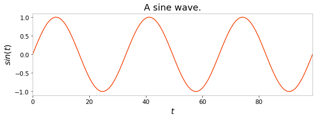
During this tutorial, we will be using the same task as introduced in the “Getting started” tutorial: we create 100 samples of a sine wave, and divide these 100 timesteps between a 50 timesteps training timeseries and 50 timesteps testing timeseries.
[2]:
import numpy as np
import matplotlib.pyplot as plt

X = np.sin(np.linspace(0, 6 * np.pi, 100)).reshape(-1, 1)

X_train = X[:50]
Y_train = X[1:51]

plt.figure(figsize=(10, 3))
plt.title("A sine wave.")
plt.ylabel("$sin(t)$")
plt.xlabel("$t$")
plt.plot(X)
plt.show()
Input-to-readout connections#
More advanced ESNs may include direct connections from input to readout. This can be achieved using the Input node and advanced features of model creation: connection chaining with the >> operator and connection merge using the & operator.

[3]:
from reservoirpy.nodes import Reservoir, Ridge, Input

data = Input()
reservoir = Reservoir(100, lr=0.5, sr=0.9)
readout = Ridge(ridge=1e-7)

esn_model = data >> reservoir >> readout & data >> readout
The & operator can be used to merge two Model together. Here, we first connect the input to the reservoir and the reservoir to the readout. As models are a subclass of nodes, it is also possible to apply the >> on models, allowing chaining. When a model is connected to a node, all output nodes of the model are automatically connected to the node. A new model storing all the nodes involved in the process, along with all their connections, is created.
connection_1 = data >> reservoir >> readout
Then, we define another model connecting the input to the readout.
connection_2 = data >> readout
Finally, we merge all connections into a single model:
esn_model = connection_1 & connection_2
A same model can be obtained using another syntax, taking advantage of many-to-one and one-to-many connections. These type of connections are created using iterables of nodes:
[4]:
esn_model = [data, data >> reservoir] >> readout
In that case, we plug two models into the readout: data alone and data >> reservoir. This is equivalent to the syntax of the first example.
[5]:
esn_model.nodes
[5]:
[Input(), Ridge(ridge=1e-07), Reservoir(units=100, lr=0.5, sr=0.9)]
Note that the same can be achieved using the ESN class seen previously, using the input_to_readout argument:
[6]:
from reservoirpy import ESN

esn_model2 = ESN(units=100, ridge=1e-7, input_to_readout=True)
Feedback connections#
Feedback connections are another important feature of ESNs. All nodes in ReservoirPy can be connected through feedback connections. Once a feedback connection is established between two nodes, the feedback receiver will receive the state of the feedback sender. When running on a timeseries, this access will hence allow the receiver to access the output of the sender, with a time delay of one timestep.
To declare a feedback connection between two nodes, you can use the << operator. This operator will create a model with a delayed connection from the right operand to the left.

Let’s add a feedback connection between our readout and our reservoir.
[7]:
from reservoirpy.nodes import Reservoir, Ridge

reservoir = Reservoir(100, lr=0.5, sr=0.9)
readout = Ridge(ridge=1e-7)

# Echo State Network with feedback
esn_model = reservoir >> readout  # regular feed-forward connection
esn_model &= reservoir << readout  # feedback (delayed) connection
Once all nodes are initialized - after training the model for instance - feedback is available:
[8]:
esn_model = esn_model.fit(X_train, Y_train)
esn_model(X[0])

print("Stored feedback:", esn_model.feedback_buffers)
Stored feedback: {(Ridge(ridge=1e-07, input_dim=100, output_dim=1), 1, Reservoir(units=100, lr=0.5, sr=0.9, input_dim=2)): array([[-1.00263582]])}
Note that the same can be achieved using the ESN class seen previously, using the feedback argument:
[9]:
from reservoirpy import ESN

esn_model2 = ESN(units=100, ridge=1e-7, feedback=True)
Forced feedbacks#
Note that adding feedback changes the training procedure: the readout needs the reservoir activity in order to fit its model, and the reservoir needs the readout output to have a proper activity. We then need teacher forcing to obtain convergence: teacher vectors \(y\) are used as feedback for the reservoir while readout is not trained.
Generation and long term forecasting#
In this section, we will see how to use ReservoirPy nodes and models to perform long term forecasting or timeseries generation.
We will take a simple ESN as an example:
[10]:
from reservoirpy.nodes import Reservoir, Ridge

reservoir = Reservoir(100, lr=0.5, sr=0.9)
ridge = Ridge(ridge=1e-7)

esn_model = reservoir >> ridge
Imagine that we now desire to predict the 100 next steps of the timeseries, given its 10 last steps.
In order to achieve this kind of prediction with an ESN, we first train the model on the simple one-timestep-ahead prediction task defined in the sections above:
[11]:
esn_model = esn_model.fit(X_train, Y_train, warmup=10)
Now that our ESN is trained on that simple task, we reset its internal state and feed it with the 10 last steps of the training timeseries.
Based on this state, we will now predict the next step in the timeseries. Then, this predicted step will be fed to the ESN again, and so on 100 times, to generate the 100 following timesteps. In other words, the ESN is running over its own predictions.
[12]:
Y_pred = np.empty((100, 1))
x = Y_train[-1]

for i in range(100):
    x = esn_model(x)
    Y_pred[i] = x
[13]:
plt.figure(figsize=(10, 3))
plt.title("100 timesteps of a sine wave.")
plt.xlabel("$t$")
plt.plot(Y_pred, label="Generated sin(t)")
plt.legend()
plt.show()
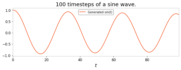
The long term forecasting ability of ESNs are one of their most impressive features. You have seen in this section how to perform this kind of generative task using a for-loop and an ESN call method.
Parallelization#
Running a model in parallel#
When we are dealing with multiple timeseries at once, a model can be run on them independently in parallel. This can be simply done by specifying the workers argument of the run method.
[14]:
# Our multi-timeseries dataset: japanese_vowels
from reservoirpy.datasets import japanese_vowels

X_train, X_test, Y_train, Y_test = japanese_vowels(repeat_targets=True)

print("Shape of the 5 first training timeseries")
print("X_train: ", [x.shape for x in X_train[:5]])
print("Y_train: ", [y.shape for y in Y_train[:5]])
Shape of the 5 first training timeseries
X_train:  [(20, 12), (26, 12), (22, 12), (20, 12), (21, 12)]
Y_train:  [(20, 9), (26, 9), (22, 9), (20, 9), (21, 9)]
[15]:
# Create a deep ESN
res1 = Reservoir(100)
res2 = Reservoir(100)
res3 = Reservoir(100)
readout = Ridge(1e-3, Wout=np.ones((300, 9)), bias=np.ones((9,)))

model = res1 >> res2 >> res3 >> readout
model &= (res1 >> readout) & (res2 >> readout)
[16]:
Y_pred = model.run(X_test, workers=4)  # Run the model on 4 different processes

print("Shape of the 5 first output timeseries")
print("Y_pred: ", [y.shape for y in Y_pred[:5]])
Shape of the 5 first output timeseries
Y_pred:  [(19, 9), (17, 9), (19, 9), (18, 9), (24, 9)]
Training a model in parallel#
Most models can also be trained in parallel in the same fashion:
[17]:
model.fit(X_train, Y_train, workers=-1) # workers=-1 to run on all available CPU cores
[17]:
Model(Reservoir(units=100, input_dim=12), Reservoir(units=100, input_dim=100), Reservoir(units=100, input_dim=100), Ridge(ridge=0.001, input_dim=300, output_dim=9))
However, while any model can be ran in parallel, this is not always true for fitting. For a model to be able to run in parallel, all of its trainable nodes must be trainable in parallel!
This is the case for the Ridge node, but not for RLS or IPReservoir for example.
State management with multiple timeseries#
When running or fitting a model on multiple timeseries at once (either by passing a 3-D array or a list of 2-D arrays, see the note on data format in the quick start guide), keep in mind the following:
The model is ran on each timeseries with the same initial state, as if there was no other timeseries.
The state of a model after being ran on multiple timeseries is that of the model only being ran on the last timeseries
This behavior has been chosen to allow for parallel processing.
Custom weight matrices#
From reservoirpy.mat_gen module#
The reservoirpy.mat_gen module contains ready-to-use initializers able to create weights from any scipy.stats distribution, along with some more specialized initializations functions.
Below are some examples:
[18]:
# Random sparse matrix initializer from uniform distribution,
# with spectral radius to 0.9 and connectivity of 0.1.

from reservoirpy.mat_gen import uniform

# Matrix creation can be delayed...
initializer = uniform(sr=0.9, connectivity=0.1)
matrix = initializer(100, 100)

# ...or can be performed right away.
matrix = uniform(100, 100, sr=0.9, connectivity=0.1)
[19]:
# Dense matrix from Gaussian distribution,
# with mean of 0 and variance of 0.5
from reservoirpy.mat_gen import normal

matrix = normal(50, 100, loc=0, scale=0.5)

# Sparse matrix from uniform distribution in [-0.5, 0.5],
# with connectivity of 0.9 and input_scaling of 0.3.
from reservoirpy.mat_gen import uniform

matrix = uniform(200, 60, low=0.5, high=0.5, connectivity=0.9, input_scaling=0.3)

# Sparse matrix from a Bernoulli random variable
# giving 1 with probability p and -1 with probability 1-p,
# with p=0.5 (by default) with connectivity of 0.2
# and fixed seed, in Numpy format.
from reservoirpy.mat_gen import bernoulli

matrix = bernoulli(10, 60, connectivity=0.2, sparsity_type="dense")
This functions can be tuned and integrated to any Node accepting initializer functions. In particular, they can be used to tune parameters distribution in a reservoir.
From Numpy arrays or Scipy sparse matrices#
In addition to initializer functions, parameters can be initialized using Numpy arrays or Scipy sparse matrices of correct shape.
[20]:
from reservoirpy.nodes import Reservoir

W_matrix = np.random.normal(0, 1, size=(100, 100))
bias_vector = np.ones((100, 1))

reservoir = Reservoir(W=W_matrix, bias=bias_vector)

states = reservoir(X[0])
From custom initializer functions#
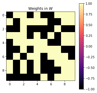
Readouts and reservoirs hold parameters stored as NumPy array or SciPy sparse matrices. These parameters can be initialized at first run of the node. This initialization is performed by calling initializer functions, which take as parameters the shape of the parameter matrix and return an array or a SciPy sparse matrix. Initializer functions can be passed as parameter to reservoirs or readouts:
[21]:
from reservoirpy.nodes import Reservoir


def bernoulli_w(n, m, **kwargs):
    return np.random.choice([-1, 1], size=(n, m))


reservoir = Reservoir(10, W=bernoulli_w)

reservoir(X[0])

plt.figure(figsize=(5, 5))
plt.title("Weights in $W$")
plt.imshow(reservoir.W)
plt.colorbar()
plt.show()
Complex architectures#
Nodes can be combined in any way to create deeper structure than just a reservoir and a readout. Connecting nodes together can be done by chaining the >> and the & operator.
The
>>operator allows to compose nodes to form a chain model. Data flows from node to node in the chain.The
&operator allows to merge models together, to create parallel pathways. Merging two chains of nodes will create a new model containing all the nodes in the two chains along with all the connections between them.
Below are examples of so called deep echo state networks, from schema to code, illustrating the use of these two operators. More extensive explanations about complex models can be found in the From Nodes to Models documentation.
Training and running on multiple reservoirs#
When training or running a model that has multiple inputs or trainable nodes, a dict (indexed by Node names) should be used to dispatch timeseries to the different nodes. Similarly, models with multiple outputs will return a dict of all the Node’s outputs.
[22]:
import numpy as np

X1 = X2 = X3 = np.sin(np.linspace(0, 12 * np.pi, 200)).reshape(-1, 1)
Y1 = Y2 = np.sin(np.linspace(0, 4 * np.pi, 200)).reshape(-1, 1)
Example 1 - Hierarchical ESN#

[23]:
from reservoirpy.nodes import Reservoir, Ridge, Input


reservoir1 = Reservoir(100, name="res1-1")
reservoir2 = Reservoir(100, name="res2-1")

readout1 = Ridge(ridge=1e-5, name="readout1-1")
readout2 = Ridge(ridge=1e-5, name="readout2-1")

model = reservoir1 >> readout1 >> reservoir2 >> readout2
This model can be trained by explicitly delivering targets to each readout using a dictionary:
[24]:
model = model.fit(X1, {"readout1-1": Y1, "readout2-1": Y2})
Example 2 - Deep ESN#

[25]:
from reservoirpy.nodes import Reservoir, Ridge, Input

data = Input(name="data")
reservoir1 = Reservoir(100, name="res1-2")
reservoir2 = Reservoir(100, name="res2-2")
reservoir3 = Reservoir(100, name="res3-2")

readout = Ridge(1, name="readout-2")

model = reservoir1 >> reservoir2 >> reservoir3 & data >> [reservoir1, reservoir2, reservoir3] >> readout

model.fit(X1, Y1)
[25]:
Model(Reservoir(units=100, input_dim=1, name=res1-2), Reservoir(units=100, input_dim=101, name=res2-2), Reservoir(units=100, input_dim=101, name=res3-2), Input(name=data), Ridge(ridge=1, input_dim=300, output_dim=1, name=readout-2))
Example 3 - Multi-inputs#

[26]:
import numpy as np
from reservoirpy.nodes import Reservoir, Ridge

reservoir1 = Reservoir(100, name="res1-3")
reservoir2 = Reservoir(100, name="res2-3")
reservoir3 = Reservoir(100, name="res3-3")

readout1 = Ridge(1, name="readout1")
readout2 = Ridge(1, name="readout2")

model = [reservoir1, reservoir2] >> readout1 & [reservoir2, reservoir3] >> readout2

model.fit(
    {"res1-3": X1, "res2-3": X2, "res3-3": X3},
    {"readout1": Y1, "readout2": Y2},
)

out = model.run({"res1-3": X1, "res2-3": X2, "res3-3": X3})
# out = {"readout1": out1, "readout2": out2}

out1 = out["readout1"]
out2 = out["readout2"]

print(out1.shape, out2.shape)
(200, 1) (200, 1)
Working with incomplete target data#
You may encounter situations where you have target data with missing values (NaN).
This case is covered by the Model.fit() and Node.fit() methods.
When training or running the model, for the steps where target values are missing, the input values will still be fed to the reservoir - thus updating the reservoir states - but the readout will not be fitted.
This property can be used to ignore target data that you do not want the readout to be trained on.
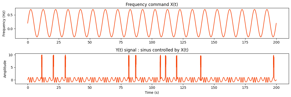
Example : signal command which corrupted target#
In this example, input data is the command for the frequency of a sine wave which will be our target data. In real life, response to command may not be perfect and there could be absurd values. We typically would not want to train our model on the corrupted values.
[27]:
# Parameters
T = 20000  # number of time steps
dt = 0.01  # temporal resolution in seconds
t = np.arange(T) * dt  # time
np.random.seed(42)  # for reproducibility
# frequency command signal X(t) :
X = 0.5 * np.sin(2 * np.pi * 0.1 * t) + 0.2

# Y response signal Y(t)
phase = 2 * np.pi * np.cumsum(X) * dt
Y = np.sin(phase)
corrupted_indices = np.random.choice(T, size=int(0.0005 * T), replace=False)
corruption_len = 50
for i in corrupted_indices:
    if i < T - corruption_len:
        Y[i : i + corruption_len] = np.random.uniform(5, 10, size=corruption_len)

plt.figure(figsize=(12, 4))
plt.subplot(2, 1, 1)
plt.plot(t, X)
plt.title("Frequency command X(t)")
plt.ylabel("Frequency (Hz)")

plt.subplot(2, 1, 2)
plt.plot(t, Y)
plt.title("Y(t) signal : sinus controlled by X(t)")
plt.xlabel("Time (s)")
plt.ylabel("Amplitude")

plt.tight_layout()
plt.show()
[28]:
from reservoirpy.nodes import Reservoir, Ridge

train_test_split = int(0.75 * T)  # 75% for training, 25% for testing
X_train = X[:train_test_split].reshape(-1, 1)
X_test = X[train_test_split:].reshape(-1, 1)
Y_train = Y[:train_test_split].reshape(-1, 1)
Y_test = Y[train_test_split:].reshape(-1, 1)

reservoir = Reservoir(100, lr=1, sr=0.9)
readout = Ridge(ridge=1e-7)
esn_model = reservoir >> readout
esn_model = esn_model.fit(X_train, Y_train)

pred = esn_model.run(X_test)
plt.figure(figsize=(12, 4))
plt.plot(t[train_test_split:], Y_test, label="True Y(t)")
plt.plot(t[train_test_split:], pred, label="Predicted Y(t)")
plt.legend()
plt.ylim(-1.5, 2)
plt.title("Predicted Y(t) vs True Y(t)")
plt.show()
[28]:
Text(0.5, 1.0, 'Predicted Y(t) vs True Y(t)')
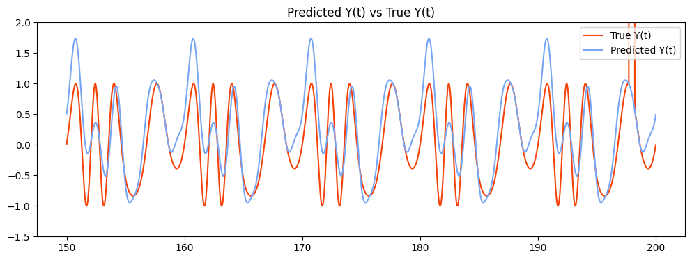
During the training, corrupted values affect how the ESN learn to predict target values.
Predicted target data here tends to have higher peaks due to the training on the corrupted target, which we do not want.
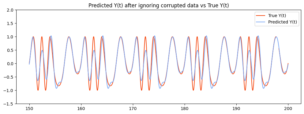
[29]:
for i in range(len(Y)):
    if Y[i] > 1 or Y[i] < -1:
        Y[i] = np.nan  # ignore corrupted data
Y_train = Y[:train_test_split].reshape(-1, 1)
Y_test = Y[train_test_split:].reshape(-1, 1)
esn_model = esn_model.fit(X_train, Y_train)
pred = esn_model.run(X_test)
plt.figure(figsize=(12, 4))
plt.plot(t[train_test_split:], Y_test, label="True Y(t)")
plt.plot(t[train_test_split:], pred, label="Predicted Y(t)")
plt.legend()
plt.ylim(-1.5, 2)
plt.title("Predicted Y(t) after ignoring corrupted data vs True Y(t)")
plt.show()
[29]:
Text(0.5, 1.0, 'Predicted Y(t) after ignoring corrupted data vs True Y(t)')